Ryan McGee
Simple Music in MATLAB
MATLAB files: proj1.m, oct.m (paste both in work directory and run proj1)
Abstract
In this project I used MATLAB to generate discrete sinusoids of one octave of musical notes using the sampling frequency of my choice. I then played back the octave at different multiples of the sampling frequency and observed the change in pitch. I continued by adding commands to control note duration and produce octave shifts without changing the sampling or reconstruction frequency. Lastly, overtones were added to each note, which I used to play back a short piece of music.
MATLAB Code With
Commentary
Setting
the Sampling and Reconstruction Frequency
|
Fs1 = 44100; %Set
Sampling Frequency Fr = Fs1; %Set
Reconstruction Frequency Fs = Fs1; % The
multiple of the sampling frequency to be used T = 1/Fs; %Sampling
Period |
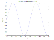
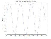
First, I chose Fs1 to be 44,100 Hz, which is the default sampling rate for most computer audio cards when recording music or sound samples. I also chose to hold the reconstruction frequency, Fr, constant at Fs1 and use Fs as the sampling frequency that I modify to produce changes in the sound. Fs = Fs1 by default so there is no change in the sound. If we set Fs = 2*Fs1 the pitch will go down an octave (cut frequency in half), and if we set Fs = 0.5*Fs1 the pitch will go up an octave (double the frequency).
|
The Standard 440 Hz A note. |
We see that when Fs is cut in half, the note frequency doubles. |
Figure 1.
Effect of Changing the Sampling Frequency on a Note
Setting Note Duration
|
N = 0.2*Fs1 % Number
of samples to achieve desired duration L = 1; %
default value for L (L=1 => no duration change) n = @(L)
1:L*N; %the array, n, takes an integer multiplier, L, that can
reduce or increase the duration of a note, i.e. 1/2 note, 1/4 note, etc |
The N variable is multiplied by a number in order to produce notes of a reasonable length in time when output to speakers. By modifying the multiplier one can effectively change the tempo of the output notes. The array, n, is a function that takes the argument, L, which scales the length of the array to result in longer or shorter note duration. L is set to 1 by default so that there is no duration change.
Generation
of Sinusoids
|
%Generate
General Sinusoid %m is
the desired octave, which is transformed into the appropriate multiplier by
the oct function %L is
the desired length of the note (in quarter notes) %fN is
the frequncy of the note note = @(m, L,
fN) sin(2*pi*oct(m)*fN*T*n(L)); %standard note at fund. freq. fA = 440.00; % Master
Tuned to A 440 fGS =
fA*2^(-1/12); fG = fGS*2^(-1/12); fFS =
fG*2^(-1/12); fF =
fFS*2^(-1/12); fE =
fF*2^(-1/12); fDS =
fE*2^(-1/12); fD =
fDS*2^(-1/12); fCS =
fD*2^(-1/12); fC =
fCS*2^(-1/12); fAS =
fA*2^(1/12); fB =
fAS*2^(1/12); |
To generate the standard sinusoid I started from a standard continuous time signal, sin(2πf), and converted it to discrete time using f = nT. I then added an octave shift function to downsample or upsample respectively. Notice that the note function takes a third argument, fN, that will determine which musical note is generated by the sinusoid. We see that the sinusoid is construced as in the following pseudocode:
Note = func. of
desired oct. and dur. = sin(2*pi*down/upsample*freq.*T*n(L));
The oct and n functions become very useful when creating music because the composer can change the octave and duration of each note on the spot without having to create all 88 notes of the standard musical keyboard. Thus, digital keyboards would only need to store 12 sound samples of each preset in their memory to be able to play all 88 notes.
Setting the Octave
|
m = 0; %default
input for oct, the octave shift function %%%%%%%%%%%%
begin oct.m%%%%%%%%%%%% function y = oct(m) if m >= 0 y = 2^m; end if m < 0 y = 1/2^(-m); end %%%%%%%%end
of oct.m%%%%%%%%%%%%%%%% |
The
variable m is the desired octave and input for the oct function which generates
the appropriate multiplier to change the octave of a note by downsampling or
upsampling. We see that the note
will be downsampled if the desired octave is greater than or equal to zero and
upsampled if the desired octave is less than zero. So, to move up one octave we enter 1 for m, which is
translated into a 2 by the oct function.
To move down one octave we enter -1, which is then translated into 0.5.
|
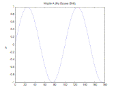
The following command plots a middle A note (440Hz) plot(n(0.04),
A(0, 0.04));
Result: The Note A at 440Hz |
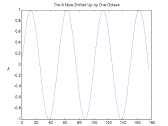
The following command plots an A note (440Hz) shifted up one octave plot(n(0.04),
A(1, 0.04));
Result: The Note A
at 880Hz |
Figure 2.
Visual Representation of an Octave Shift Using Downsampling
By moving up one octave using downsampling we see twice as many cycles of the A waveform within the same number of samples, which tells us that the output frequency has doubled to 880 Hz. Notice that downsampling has the same effect on the note as changing the sampling frequency. Hence, the advantage of downsampling is that it lets us modify pitch without changing the sampling or reconstruction frequency.
Generation
of Musical Notes with Overtones
|
namp = 1; % set
the amplitude for the natural freq hamp = 0.8; % set
the amplitude for the overtones %each
note passes m and L to the note function above %two
overtones are added to each note C = @(m, L)
namp*note(m, L, fC) + hamp*note(m, L, 0.5*fC) + hamp*note(m, L, 2*fC); CS = @(m, L)
namp*note(m, L, fCS) + hamp*note(m, L, 0.5*fCS) + hamp*note(m, L, 2*fCS); D = @(m, L)
namp*note(m, L, fD) + hamp*note(m, L, 0.5*fD) + hamp*note(m, L, 2*fD); DS = @(m, L)
namp*note(m, L, fDS) + hamp*note(m, L, 0.5*fDS) + hamp*note(m, L, 2*fDS); E = @(m, L)
namp*note(m, L, fE) + hamp*note(m, L, 0.5*fE) + hamp*note(m, L, 2*fE); F = @(m, L)
namp*note(m, L, fF) + hamp*note(m, L, 0.5*fF) + hamp*note(m, L, 2*fF); FS = @(m, L)
namp*note(m, L, fFS) + hamp*note(m, L, 0.5*fFS) + hamp*note(m, L, 2*fFS); G = @(m, L)
namp*note(m, L, fG) + hamp*note(m, L, 0.5*fG) + hamp*note(m, L, 2*fG); GS = @(m, L)
namp*note(m, L, fGS) + hamp*note(m, L, 0.5*fGS) + hamp*note(m, L, 2*fGS); A = @(m, L)
namp*note(m, L, fA) + hamp*note(m, L, 0.5*fA)+ hamp*note(m, L, 2*fA); AS = @(m, L)
namp*note(m, L, fAS) + hamp*note(m, L, 0.5*fAS) + hamp*note(m, L, 2*fAS); B = @(m, L)
namp*note(m, L, fB) + hamp*note(m, L, 0.5*fB) + hamp*note(m, L, 2*fB); |
To produce a more natural sound I added two overtones to each note. Each note is a sum of three instances of the general sinusoid defined earlier. The first instance is the note played at its standard frequency in the desired octave input by the user. The last two instances are the note played at one octave below and one octave above the input octave. Each instance is multiplied by either namp to set the amplitude of the natural frequency or hamp, which sets the amplitude of the harmonic frequencies. By modifying the values of namp and hamp one can create different mixtures of natural frequencies and overtones, which is similar to what happens when you pluck a string or create a note through physical vibration. Thus, by adding even more overtones and properly tweaking the mixture it becomes possible to model physical instruments in the digital domain.
|
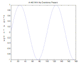
The following command plots the middle A note (440Hz) with no overtones. hamp = 0; plot(n(0.04),
A(0, 0.04));
Result:
Simple Sinusoid with a period of 100 samples |
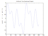
The following command plots the middle A note (440Hz) with two overtones. hamp = 0.8; plot(n(0.04),
A(0, 0.04));
Result: A more complex periodic function with a period of
200 samples |
Figure 3.
Visual Representaion of Overtones in a Note
We see that when harmonics are added the period of the tone changes to the largest period of its harmonics.
Playing Back a Composition
|
%Define
Rests er = zeros(1,
.125*N); % eigth rest qr = zeros(1,
.25*N); % quarter rest hr = zeros(1,
.5*N); % half rest tr = zeros(1,
.75*N); % three-quarter rest wr = zeros(1,
N); % whole rest %Jingle
Bells %note(octave,
duration in 1/4 notes) example: A=C(1,1) = 1/4 note middle C jbseq1 =
[A(0,1) qr A(0,1) qr A(0,2) qr]; jbseq2 =
[A(0,1) qr C(1,1) qr F(0,1) qr G(0,1) qr A(0,4) qr]; jbseq3 =
[AS(0,1) qr AS(0,1) qr AS(0,1) qr AS(0,0.5) qr AS(0,1) qr A(0,1) qr A(0,1) qr
A(0,0.5) er A(0,0.5) qr A(0,1) qr G(0,1) qr G(0,1) qr A(0,1) qr G(0,2) qr
C(1,2) qr]; jbseq4 =
[AS(0,1) qr AS(0,1) qr AS(0,1) qr AS(0,1) qr AS(0,1) qr A(0,1) qr A(0,1) qr
A(0,0.5) er A(0,0.5) qr C(1,1) qr C(1,1) qr AS(0,1) qr G(0,1) qr F(0,4)]; jbseq5 = [C(0,1)
qr A(0,1) qr G(0,1) qr F(0,1) qr C(0,3) qr C(0,0.5) er C(0,0.5) qr C(0,1) qr
A(0,1) qr G(0,1) qr F(0,1) qr D(0,4) qr]; jbseq6 =
[D(0,1) qr AS(0,1) qr A(0,1) qr G(0,1) qr E(0,4) qr C(1,1) qr C(1,1) qr
AS(0,1) qr G(0,1) qr A(0,4) qr]; jbseq7 =
[C(0,1) qr A(0,1) qr G(0,1) qr F(0,1) qr C(0,4) qr C(0,1) qr A(0,1) qr G(0,1)
qr F(0,1) qr D(0,4) qr]; jbseq8 =
[D(0,1) qr AS(0,1) qr A(0,1) qr G(0,1) qr C(1,1) qr C(1,1) qr C(1,1) qr
C(1,0.5) er C(1,0.5) qr D(1,1) qr C(1,1) qr AS(0,1) qr G(0,1) qr F(0,1) wr
C(1,2) qr]; jbseq9 =
[AS(0,1) qr AS(0,1) qr AS(0,1) qr AS(0,1) qr AS(0,1) qr A(0,1) qr A(0,1) qr
A(0,0.5) er A(0,0.5) qr C(1,1) qr C(1,1) qr AS(0,1) qr G(0,1) qr F(0,4) qr ]; %Song
constructed from several, sometimes repeating, jbsequences jbells =
[jbseq1 jbseq1 jbseq2 jbseq3 jbseq1 jbseq1 jbseq2 jbseq4 jbseq5 jbseq6 jbseq7
jbseq8 jbseq1 jbseq1 jbseq2 jbseq3 jbseq1 jbseq1 jbseq2 jbseq3 jbseq9]; %Output
song reconstructed at Fr sound(0.25*jbells,
Fr); % the multiplier in front of song sets the master volume |
If four C quarter notes are to be played in a bar of music a
pianist knows to press the C key four times equally spaced to create the
appropriate rhythm. However, if MATLAB sees four C quarter notes it will play
them as one continuous note rather than four equally spaces notes. Thus, a quarter rest in my code does
not directly correspond to a quarter rest in actual music. My quarter rest, qr, is used as the
default spacing between notes in order to give rhythm to the song. If an actual quarter rest is required
in the music then I would use a whole rest, which is the same length as a quarter
note, N. If a true whole rest was
required then I would simply use four whole rests. This problem can be fixed by adding a release property to
the notes along with the attack, decay, and sustain properties found on most
synthesizers.
To simplify the composition process I divided the song into several
sequences so I could play them back one at a time until they were ready to be
added together in the song vector, jbells. Also, several of the sequences repeated in the song, which
significantly reduced the amount of notes for me to input.
Lastly, the song is output at Fr using the sound command and
a multiplier in front of the song vector in order to control the volume level.
(While Jingle Bells does not include several instances of
octaves other than 0, I have also prepared a vector that plays all notes from
C(-2) to B(2) for demonstration purposes.)
CONCLUSION
This project was an interesting first step into the musical
capacity of MATLAB. I believe that
would be very possible to model an instrument or create a synthesizer with
MATLAB. Adding envelopes, filters,
and a step sequencer could make for a decent digital music production
tool. Several music languages such
as Csound already exist, but do not require as deep an understanding of
mathematics and programming methods.
Thus, further exploration of music in MATLAB could produce ways for
musicians to obtain signal processing and programming skills, while engineers
and programmers could use their technical skills to better understand
music.
(Equally plausible may the capacity of LabVIEW for music, for it allows easy GUI development and has a programming style similar to Max/MSP.)
